Open-source Julia packages for first-order optimization
This was originally posted here on BlackRock’s engineering blog.
In this post, we present two Julia packages that the BlackRock AI Labs has released, PiecewiseQuadratics.jl and SeparableOptimization.jl, along with a new Julia organization we created that is dedicated to first-order optimization methods. We originally developed these packages and the corresponding methodology to solve a class of portfolio construction problems, which we detail in a paper published in March. We will feature this work in a talk at the JuliaCon 2021 JuMP-dev workshop later this month!
See also: another implementation of these packages in Rust, as described in this blog post.
Why Julia?
After devising the ADMM based optimization methodology described in the paper, there was no question what language we would use to implement it. Julia’s unparalleled combination of an elegant and expressive high-level syntax with C/Fortran level speed allowed us to quickly translate our formulations into efficient code. We are excited to share it with the growing Julia optimization community!
PiecewiseQuadratics.jl
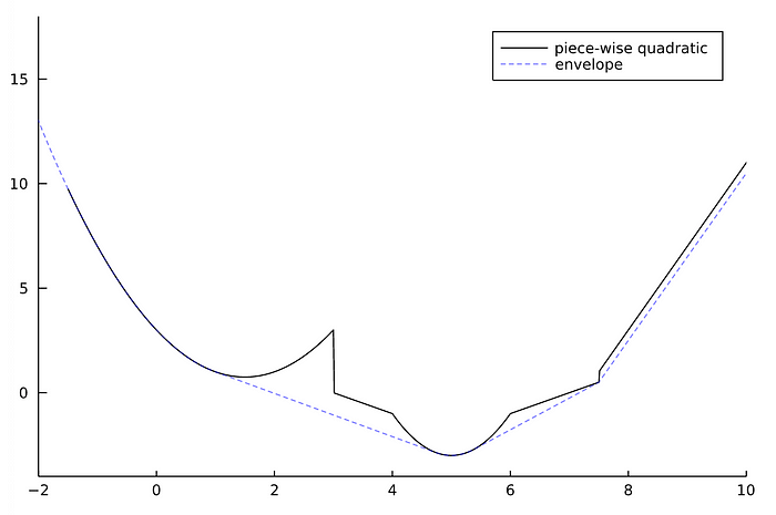
This package allows for the representation and manipulation of univariate piecewise quadratic functions, designed to be used as a cost function in optimization packages. Piecewise quadratic functions are composed of several equations (“pieces”), each of which takes the standard quadratic form and applies to a different part of the domain. Consider the following example:
\[f(x) = \left\{\begin{array}{ll} x^2 - 3x - 3 & \text{if } x \in [-\infty, 3]\\ x + 3 & \text{if } x \in [3, 4]\\ 2x^2 - 20x + 47 & \text{if } x \in [4, 6]\\ x - 7 & \text{if } x \in [6, 7.5]\\ 4x - 29 & \text{if } x \in [7.5, \infty]\\ \end{array}\right.\]Within PiecewiseQuadratics.jl, we would represent f as a PiecewiseQuadratic, which is simply a list of BoundedQuadratics. Here, each BoundedQuadratic represents our quadratic equation “pieces,” and is defined by the equation’s p, q, and r terms along with the Interval it applies to (represented by [lb, ub]). Altogether, we represent f with the following code:
f = PiecewiseQuadratic([
    # BoundedQuadratic(lb, ub, p, q, r),
    BoundedQuadratic(-Inf, 3.0, 1.0, -3.0, 3.0),
    BoundedQuadratic(3.0, 4.0, 0.0, -1.0, 3.0),
    BoundedQuadratic(4.0, 6.0, 2.0, -20.0, 47.0),
    BoundedQuadratic(6.0, 7.5, 0.0, 1.0, -7.0),
    BoundedQuadratic(7.5, Inf, 0.0, 4.0, -29.0)
])
Note: although this function is complete over the domain, this is not a requirement! Functions default to Inf when evaluated on undefined segments.
We implement several methods that are useful for optimization — such as the sum, the derivative, the convex envelope, and the prox operator — as well as several utility methods. Below we visualize the function f that we previously defined along with its convex envelope using get_plot (which allows interfacing with your favorite Julia plotting library) and JuliaPlots:
using Plots
plot(get_plot(f); label="piece-wise quadratic", grid=false, color=:black)
plot!(get_plot(simplify(envelope(f))); label="envelope", linestyle=:dash, color=:blue, la=0.5)
See the PiecewiseQuadratics.jl documentation for details and more examples of the package!
SeparableOptimization.jl
This package uses a derivative of ADMM to solve Linearly Constrained Separable Optimization (LCSO) problems. LCSO problems have cost functions that are separable over the decision variable and have linear constraints. In our portfolio construction example, the decision variable is a vector, where the entries are the percent of our total portfolio value in each of assets; we require that these values sum to (a linear constraint) and add in cost functions that are specific to each asset (they separate over our decision variable). These costs could be anything from a cost to hold each asset (e.g., the cost to short TSLA is higher than for MSFT), to position limits per asset (e.g., requiring 10–20% of our portfolio value is in BTC), to combinations of various other costs. Often these functions are very complicated — we represent them using PiecewiseQuadratics.jl!
LCSO problems are a very general formulation and have wide application beyond portfolio optimization. Other applications might include radiation treatment planning — where we optimize the radiation intensity pattern for cancer treatment — or dynamic energy management — where we optimize the power usage of a network of devices over time.
See the paper for more information on LCSO problems and our portfolio construction example, and the SeparableOptimization.jl documentation for details and examples of the package!
A new Julia organization
In the process of open sourcing these packages, we thought a lot about how to maximize their impact and usage. Julia’s open-source community often organizes around GitHub Organizations.
“This allows for a higher degree of collaboration and structure that ultimately enables each of these communities to be self-sustaining.”
Rather than hosting these packages on BlackRock’s GitHub, we wanted to find an organization to host them alongside other related packages that would be of mutual benefit. After discussion with various organizations, we realized that there were a few related packages out there, but no organization dedicated to first-order optimization methods. So, we decided to create JuliaFirstOrder. We currently have five packages and are actively working to cultivate the community. A special thank you to Miles Lubin for sparking the idea and making the right introductions!
Conclusions
We are very excited to get these new packages into the hands of the Julia community, and to grow our new organization. Head to their documentation pages to learn more and how to give them a try. Don’t forget to tune into our presentation at JuliaCon 2021 titled “Linearly Constrained Separable Optimization!”